October 1, 2025 by S. Rennie
Unlocking Insight from Complex Survey Data

In today’s data‑driven landscape, the ability to transform raw, messy datasets into reliable, analysis‑ready assets is a critical competitive advantage.
The Australian Marriage Law Postal Survey 2017 1, released by the Australian Bureau of Statistics (ABS), offers a perfect case study. Its Excel workbook contains six distinct tables, each with its own structure, merged cells, and embedded notes. Below we walk through a systematic, reproducible workflow that cleans, validates, and consolidates this information into a single, tidy CSV file ready for downstream analytics.
Understanding the Source
The original workbook comprises:
| Sheet | Content |
|---|---|
| Contents | Non‑data metadata |
| Table 1–3 | Participation by State & Territory (overall, males, females) |
| Table 4–6 | Participation by Federal Electoral Division (overall, males, females) |
| Explanatory Notes | Non‑data metadata |
Key challenges:
- Mixed granularity: State‑level vs. electoral‑division level.
- Merged cells: State names appear only once per block.
- Redundant “total” rows/columns: Calculated sums that sometimes conflict with raw data.
- Embedded footnotes: Extraneous rows that must be stripped.
Preparing the Workbook
A Jupyter Notebook was used for this project with a custom T3Data kernel installed. The Workbook was read into the Notebook and the six data tables extracted:
import pandas as pd
import numpy as np
import utils # Custom T3Data helper functions

xlsx = pd.ExcelFile('datasets/examples121/australian_marriage_law_postal_survey_2017_-_participation_final.xls')

used_sheets = xlsx.sheet_names[1:-1]   # Drop “Contents” and “Explanatory Notes"
Cleaning the Sheets
As there were two different table styles, two different cleaning methods were required.
Cleaning the State‑Level Tables (Sheets 1‑3)
Steps performed on each sheet:
- Read with proper header: header=5 skips introductory rows.
- Rename generic columns:
Unnamed: 0 → State,Unnamed: 1 → Metric. - Drop trailing notes: The final seven rows contain explanatory text.
- Fill missing state names: Forward‑fill (
ffill) propagates the merged cell value. - Set a MultiIndex:
(State, Metric)makes subsequent slicing intuitive. - Append to a list: Each cleaned DataFrame is stored for later concatenation.
Result: a tidy table where each row uniquely identifies a state and a metric (e.g., “Eligible participants”).
Cleaning the Electoral‑Division Tables (Sheets 4‑6)
These sheets require extra handling because the first column holds the electoral division, while the state name appears only on merged header rows.
An extra step was required to create a new column where each row had the State name, only if the metric column was empty (true for all merged header rows):
# Copy State name to new column before filling down to subsequent rows
state = sheet_df['Electoral Division'].where(sheet_df['Metric'].isna())
sheet_df.insert(0, 'State', state)
sheet_df['State'] = sheet_df['State'].ffill()
Normalizing Indexes
When examining the DataFrame after completing the cleaning steps, it became apparent that whilst the multi-level index helped the readability and examination, it was not an appropriate. The data help in the multi-level index would be required later so it was reset:
for sheet in df:
    sheet.reset_index(inplace=True)
Removing Redundant Totals
The original sheets contain a number of derived rows and columns:
- Electoral division total rows
- Total persons columns
- Participation rate
By eliminating these, the raw data will remain. For example:
# Drop any column whose name contains “Total”
dropped_df = [sheet.drop(sheet.filter(regex='Total'), axis=1) for sheet in df]

# Drop any row whose value contains "Total" in the Electoral Division sheets
[sheet.drop(sheet[sheet['Electoral Division'].str.contains('Total')].index,
            inplace=True) for sheet in dropped_df[3:6]]

# Remove rows with “Participation rate (%)” metric
[sheet.drop(sheet[sheet['Metric'] == 'Participation rate (%)'].index,
            inplace=True) for sheet in dropped_df]
Periodic Testing
Regular testing is crucial when completing projects like this, something that is easier to do with a cleaner dataset than the original. On one of these tests, it was discovered that the original dataset had some inconsistencies when comparing against the provided ‘Total’s columns, since removed.
As can be seen below, despite the column totals being correct, the final ‘Total’ column did not match with the raw data totals. The legend for the four main highlighted sections is:
- Yellow: The original data
- Light green: The calculated ’total participants’ for each age group
- Green: The difference between the original data and calculated totals
- Red: The difference between the original data total and the calculated total
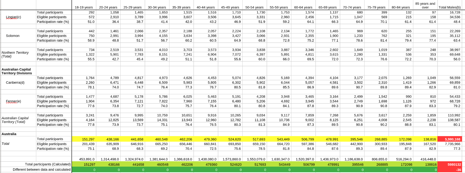 Dataset inconsistencies
Collating
Whilst completing this project, it was noticed that the first three sheets (State-wide) didn’t hold any unique data that wasn’t present in the second three sheets (Electoral divisions). By adding in the gender of participants, a final column could be added and then the final three sheets could be collated to have a clean and presentable dataset for further analysis.
The final step before collating the sheets was to add in the gender to the sheets. The ‘Total’ gender was added to retain the information contained in the overall sheet (Sheet 4) for checking and a new DataFrame was created, leaving the previous DataFrame intact for checks.
# Add in the Gender column and populate
dropped_df[3].insert(2, "Gender", "Total")   # Table 4 (overall)
dropped_df[4].insert(2, "Gender", "Male")    # Table 5 (male)
dropped_df[5].insert(2, "Gender", "Female")  # Table 6 (female)

# Combine the sheets into a new DataFrame
combined_df = pd.concat(dropped_df[3:6])

# Sort the values to retain a similar format to the original
combined_df.sort_values(['State', 'Electoral Division', 'Gender', 'Metric'],
                        inplace=True)
The resulting DataFrame contains 900 rows and 20 columns, each representing a unique combination of state, division, gender, and metric across all age brackets.
Exporting the Clean Dataset
combined_df.to_csv('raw_data.csv', index=False)
The CSV file now serves as a single source of truth for any downstream analysis, whether visualizing participation trends, modelling demographic effects, or integrating with other policy datasets.
Key Takeaways for Business Practitioners
| Technique | Why It Matters |
|---|---|
| Selective Sheet Loading | Avoids unnecessary memory overhead and focuses effort on relevant data only. |
| Header Alignment & Column Renaming | Guarantees that downstream code references meaningful names, reducing bugs. |
| Forward‑Filling Merged Cells | Restores hierarchical context lost during export, essential for accurate grouping. |
| Multi‑Level Indexing | Provides powerful slicing (e.g., “all NSW divisions”) without manual filtering. |
| Explicit Removal of Derived Columns | Keeps the dataset “raw”, ensuring calculations are traceable and testable. |
| Automated Consistency Checks | Detects subtle transcription errors (e.g., mismatched totals) before they propagate. |
| Modular Pipeline (list of DataFrames) | Enables versioned snapshots of each cleaning stage, a best practice for data governance. |
| Final Consolidation & Export | Delivers a clean, flat file that integrates seamlessly with BI tools, statistical packages, or machine‑learning pipelines. |
Closing Thoughts
Cleaning and collating data from heterogeneous sources is rarely glamorous, yet it is the foundation upon which trustworthy insights are built. By applying disciplined, reproducible steps, exactly as demonstrated with the Australian Marriage Law Postal Survey, you turn a tangled Excel workbook into a high‑quality analytical asset.
This methodology scales to any multi‑sheet, multi‑granularity dataset, empowering analysts, data engineers, and decision makers to focus on what the data tells us, rather than how to wrestle it into shape.